FEATURE ENGINEERING
(I) Azure and User Level Analysis
Diagram: Enriched User Data
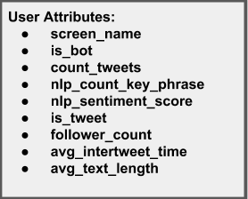
While the data collection and data cleaning was focused on tweets, we pursued one path of analysis that focused on engineering user related fields, derivied from the underlying tweet data (that contained the Azure NLP attributes) for each user. To perform this step, we grouped the de-normalized tweet-user data structure by screen_name and aggregated fields as described below to create the user level features on which we did the modeling:
- count_tweets: This attribute contains the total of the number of tweets per user. We discuss in our conclusion and future consideration potential bias introduced by this attribute and better ways to handle in the future.
- nlp_count_key_phrase: This attribute contains the mean of the count of the key phrases in each tweet per user.
- nlp_sentiment_score: This attribute contains the mean of the sentiment score of each tweet per user.
- is_tweet percent: This attribute contains the ratio of tweets to re-tweets for each user.
- follower_count: This attribute contains the total followers for each user. To clarify, the code takes the mean of the field from each tweet-user row. But, the field within each row is already the total followers per user. So, the mean of the same total in each row is the total.
- avg_intertweet_time: This attribute contains a good approximation of the standard deviation of the time between tweets (measured as a percent of an hour) for each user. The attribute was calculated using in the groupby’s aggregate method using a function we wrote called ‘calculate_avg_delta’. As with the field name, this function is mis-labeled as the function really does return the standard deviation of the distribution of delta times between tweets, not the average.
- avg_text_length: This attribute contains the mean of the lenght of the text in each tweet per user.
Below is the code snippet for generating these features:
tweet_df_grouped_user = tweet_df.groupby(['screen_name']).agg({
    'screen_name' : np.min,
    'id': 'count',
    'is_bot' : np.min,
    'nlp_count_key_phrases': np.mean,
    'nlp_sentiment_score': np.mean,
    'is_tweet': np.mean,
    'followers_count' : np.mean,
    'created_at' : calculate_avg_delta,
    'text' : calculate_avg_tweet_length
}).rename(columns={
    'id': 'count_tweets',
    'created_at' : 'avg_intertweet_time',
    'text' : 'avg_text_length'
})

def calculate_avg_delta (x):
    '''Function to generate inter-tweet feature for each user.'''
    x_sorted = np.sort(x)
    total_items = len(x)

    #return large number for user with just one Tweet
    if total_items == 1:
        return 24 * 60; # return one day

    array_deltas = np.zeros(total_items)
    one_hour_delta = np.timedelta64(1, 'h')

    for (i, item) in enumerate(x_sorted):
        if i != (total_items - 1):
            d1 = item
            d2 = x_sorted[i + 1]
            array_deltas[i] = (d2-d1) / one_hour_delta

    return np.std(array_deltas)

def calculate_avg_tweet_length (x):
    '''Function to calculate average tweets text size for each user.'''
    array_deltas = [len(item) for item in x]
    return np.mean(array_deltas)
(II) NLTK and Tweet Level Analysis
Another path we pursued, was to analyze the tweets with the NLTK API. Two key parameters were engineered for this branch of analysis: the average length of the tweets per user, and the 10 most bot-favored word choices per user.
- mean_tweet_length The tweet dataframe required too key features to engineer this feature: the tweet-user’s name and their tweets. The following line of code captures this exact feature:
# Assuming the data has already been loaded as 'text_data'

# Tokenizer breaks tweet down into str objects inside lists.
from nltk.tokenize import TweetTokenizer
tt = TweetTokenizer()

# Remove NAs
text_data.dropna(subset=['text'], inplace=True)

# Turn tweets into lists of str objects
text_data['tokens'] = text_data['text'].apply(tt.tokenize)

# Count the strings in the list
text_data['tweet_length'] = text_data['tokens'].str.len()

# Aggregate by name, compute the mean tweet lengths, and sort!
text_data.groupby(['name']).tweet_length.mean().sort_values(ascending=False)
- Top 10 Words used (10 Columns) The next objective is to identify the top 10 most frequently used words by bots. This process involves clustering all tweets [tokens] used by each user, removing stopwords (‘the’, ‘they’, ‘it’, etc.), and counting the frequencies.
# Assuming the data has already been loaded as 'text_data'

# FreqDist is a powerful tool to count frequency of strings
# stopwords is a collection of stop-words in the nltk library
from nltk import FreqDist
from nltk.corpus import stopwords
import string

# This was an earlier step to segregate the data by user-type
bot_texts = text_data.loc[text_data.known_bot == True][useful_cols]
real_texts= text_data.loc[text_data.known_bot == False][useful_cols]

# cluster words by twitter name
bot_words = bot_texts.groupby(['name']).tokens.agg(sum)
usr_words = real_texts.groupby(['name']).tokens.agg(sum)

# Clean up the two arrays created above: insert into dataframes, label, and remove stopwords
bot_words = pd.DataFrame(bot_words)
usr_words = pd.DataFrame(usr_words)

bot_words.columns = ['words']
usr_words.columns = ['words']

stop_words  = stopwords.words('english') + list(string.punctuation) + [' ','rt',"\'", "...", "..","`",'\"', '–', '’', "I'm", '…','""','“','”']

# Construct list of cleaned words
usr_words['cleaned_words'] = [[word for word in words if word.lower() not in stop_words]
                                for words in usr_words['words']]
bot_words['cleaned_words'] = [[word for word in words if word.lower() not in stop_words]
                              for words in bot_words['words']]

# Find the frequency of the cleaned_words (words with stopwords removed) per all users in the two groups.
freq_per_usr = FreqDist(list([a for b in usr_words.cleaned_words.tolist() for a in b]))
freq_per_bot = FreqDist(list([a for b in bot_words.cleaned_words.tolist() for a in b]))

# Most common words, clean
common_words_bot = pd.DataFrame(freq_per_bot.most_common())
common_words_usr = pd.DataFrame(freq_per_usr.most_common())
cols = ["Words", "Count"]
common_words_bot.columns = cols
common_words_usr.columns = cols

# Find the frequency of each word used
common_words_usr['Frequency'] = common_words_usr['Count']/len(common_words_usr)
common_words_bot['Frequency'] = common_words_bot['Count']/len(common_words_bot)

# Remove the small (len(word)<2) words which could be nonsense (emojis, 'hi', etc)
filter1 = (common_words_usr['Words'].str.len()>=3)
filter2 = (common_words_bot['Words'].str.len()>=3)
filtered_usr = common_words_usr.loc[filter1]
filtered_bot = common_words_bot.loc[filter2]
The filtered_usr/bot lists are the most used ‘important’ words in our tweet collections. Next the top 10 bot words shall be selected. Columns will be constructed for these words in the original dataframe (text_data), defaulted to 0 indicating the word has never been used.
naughty_words = filtered_bot[:10]

# Set these to 0
for word in naughty_words['Words']:
    text_data[word] = 0

# Count the instances at which these words occur across all tokens
for word in naughty_words['Words']:
    text_data[word] = text_data.apply(lambda row: row['tokens'].count(word), axis=1)


#   IMPORTANT!
# Now the word-use frequency is calculated per user.
# This is important to do because there are more bots than real people in this collection; in order to provide proportionate datasets, the frequency at which these words are uttered by that specific user in their tweers are more important than the total number of times they mention it.
# Consider this:
# Person A debating politics vs Person B shouting "trump trump trump trump": while the Person A debating politics may mention trump more than Person B, person A is using that word less frequently (perhaps in lieu for an actual conversation rather than spam).

# Sum all of the instances these select words were used by each twitter user. Also merge in the known_bot status (soon to be the endogenous variable).
text_by_names = text_data.groupby(['name']).sum()[naughty_words['Words']]
to_join = text_data[['name','known_bot']].drop_duplicates().set_index('name')
text_by_names=text_by_names.join(to_join, how='inner').drop_duplicates()

# To identify the frequency at which these words are used by the twitter user, we need to know how long their average tweets are
bot_texts2 = text_by_names.loc[text_by_names.known_bot == True].join(tweet_len_by_bot, how='inner')
usr_texts2= text_by_names.loc[text_by_names.known_bot == False].join(tweet_len_by_usr, how='inner')

# Remember: if it sounds like a bot it might just be a bot.

for word in naughty_words['Words']:
    usr_texts2[word+"_freq"] = usr_texts2[word]/usr_texts2['mean_tweet_length']
    bot_texts2[word+"_freq"] = bot_texts2[word]/bot_texts2['mean_tweet_length']
The next step is to scale the important data and separate into training and test data.
# sklearn provides excellent modules on breaking data into train/test sets, and a scaling function.
from sklearn.model_selection import train_test_split
from sklearn.preprocessing import MinMaxScaler

# Preserving important columns for labeling
cols = list(naughty_words['Words']+"_freq")
cols.append("known_bot")
cols.append('mean_tweet_length')

# Binding the bots and real users
all_res = bot_texts2.append(usr_texts2)
all_res = all_res[cols]

# Separating into train-test sets
X_train, X_test = train_test_split(all_res, test_size=.2, stratify=all_res['known_bot'])

# Extract our endogenous variable, make it binary (0's [false, not a bot] 1's [true, a bot])
y_train = X_train['known_bot']*1
y_test = X_test['known_bot']*1

# Preserving important columns for labeling
cols = list(naughty_words['Words']+"_freq")
cols.append("mean_tweet_length")

# Drop our endogenous variable from our exogenous variables.
X_train = X_train.drop('known_bot', axis=1)
X_test = X_test.drop('known_bot', axis=1)

# Scale!
scaler = MinMaxScaler().fit(X_train)
X_train = pd.DataFrame(scaler.transform(X_train))
X_test = pd.DataFrame(scaler.transform(X_test))

# Label the columns
X_train.columns = cols
X_test.columns = cols
And now the data is ready for the custom NLP processing!